

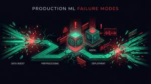
Here is the uncomfortable truth: most ML failures in production are not model problems. They are system problems. The model that hit 95% accuracy in your notebook will silently degrade to 60% in production — and you may not notice for months.
This article covers five failure modes that account for the majority of production ML incidents across CV, trading, fraud, RAG, and recommendation systems — with a PSI drift simulator, domain-frequency breakdown, and a pre-launch readiness checklist at the end.
For the specific mechanics of distribution mismatch and PSI-based detection, see the deep dive on model skewing in production. For why the web-service mental model causes most of these failures in the first place, see applied AI is not a web service.
Key Takeaways
- Most production ML failures happen in system layers — data pipelines, feature engineering, monitoring coverage — not in the model weights themselves.
- Training-serving skew (different preprocessing code paths, stale feature stores, timezone bugs) is the most insidious failure mode: it creates day-one mismatch before any drift occurs.
- Aggregate accuracy metrics hide segment failures. A model can hold 88% overall while failing at 51% on a high-value cohort. Always monitor by slice.
- Ownership ambiguity turns 2-hour incidents into 3-day incidents. Define who gets paged for what before an incident, not during it.
- A working fallback is more valuable than a perfect model without one. Graceful degradation must be designed in, not bolted on.
I. Why models degrade in production
Production degradation comes down to one root cause: the environment stops matching the assumptions the model was trained under. Data gets messier, feature pipelines diverge, monitoring stays focused on infrastructure instead of model health, ownership is fuzzy, and rollout conditions expose edge cases that offline evaluation never saw.
Understanding these failure modes is essential for anyone building production AI systems. This is also why applied AI is fundamentally different from a web service — it fails in ways that traditional software monitoring won’t catch.
Most production degradation fits one of five buckets. Those buckets are broad enough to explain why models fail after deployment across CV, trading, recommendation, fraud, and RAG systems.
II. The five failure modes
Failure Mode 1: Data quality degradation
Your model was trained on clean, curated data. Production data is messy, incomplete, and constantly changing.
Common symptoms:
- Missing fields that were always present in training
- New categories appearing in categorical features
- Numeric distributions shifting outside training ranges
- Upstream system changes breaking implicit data contracts
How to detect it: Set schema validation at ingestion. Any field that was non-null in training but has a null rate above 1% in production is a signal. Monitor feature completeness as a pipeline health metric, not just model accuracy.
Real example: A CV pipeline at AgrigateVision collapsed in the field because a camera firmware update changed image preprocessing parameters — the model had never seen the new image characteristics. No code changed on our side. The upstream hardware vendor pushed an update.
The lesson: you don’t control every input source. Your monitoring must catch changes you didn’t make.
Failure Mode 2: Pipeline drift
The silent killer. Your data pipelines change, your feature engineering evolves, but your model expects the old format.
Warning signs:
- Feature values fall outside expected ranges
- Null rates increase unexpectedly
- Processing time spikes without model changes
- A/B tests show inconsistent results across cohorts
How to detect it: Version your feature transformations. Log the actual feature values that go into the model at inference time, not just the raw inputs. Compare feature distributions between training snapshots and live data using PSI — see model skewing and data skew for a detailed breakdown of detection methods.
Typical root cause: A data engineer updates a normalization function to fix a legitimate bug. The new version produces slightly different values. The model was trained on the old values. Accuracy drops 8% over the following two weeks — and nobody connects it to the pipeline change from three weeks ago.
Failure Mode 3: Monitoring gaps
You can’t fix what you can’t see. Most teams monitor infrastructure (CPU, memory, response time) but not model health.
What you actually need to monitor:
- Input distribution: Are production inputs similar to training? Use PSI per feature, not just a global drift score.
- Prediction distribution: Is the model outputting expected score patterns? Sudden changes in output histograms are an early warning.
- Performance metrics: Accuracy, precision, recall on live data (requires ground truth labels with reasonable lag).
- Business metrics: The actual outcomes you care about — conversions, fraud caught, churn prevented.
The trap: A model can maintain 88% overall accuracy while failing on a high-value segment at 51% accuracy. Aggregate metrics hide slice-level failures — always monitor by segment, not just globally.
Failure Mode 4: Ownership ambiguity
When the model breaks at 2 AM, who gets paged? ML systems span data engineering, ML engineering, and platform teams. Without clear ownership, issues fall through cracks.
Questions that must be answered before launch:
- Who owns the training pipeline?
- Who owns the serving infrastructure?
- Who owns data quality from upstream teams?
- Who is accountable for model performance in production?
- Who gets paged for a prediction accuracy alert vs. a latency alert?
The cost of ambiguity: An incident that a clear owner would resolve in 2 hours can drag for 3 days when nobody knows who should act. In trading systems like Steve, that ambiguity has direct, immediate financial cost. In fraud detection, it means every missed fraud event in that window is a real loss.
Ownership doesn’t mean one person knows everything. It means one person is accountable for ensuring the right people are coordinated. That distinction matters at 3 AM.
Failure Mode 5: Training-serving skew
The model sees different data in production than it did during training. This is surprisingly common and notoriously hard to debug because the model doesn’t throw an error — it just quietly underperforms.
Sources of skew:
- Different preprocessing code paths (Python in training, Java in serving)
- Stale features from slow-updating feature stores
- Time-based features with timezone bugs
- Different library versions in training vs. serving environments
- Null handling differences (drop vs. fill with zero)
How to detect it: Log the actual feature vector at inference time. Periodically compare a sample of live feature vectors against your training distribution using PSI. Any feature with PSI > 0.25 is a candidate for skew investigation.
Use the simulator below to build intuition for how PSI behaves as drift grows over time:
For a deep-dive into detection methods, PSI thresholds, and architectural fixes, see Model Skewing in Production.
III. Domain-specific failure patterns
Different domains have unique failure modes beyond the generic five. Knowing domain-specific patterns lets you build targeted defenses before they surface in production.
Computer Vision failures
CV pipelines fail when input conditions change in ways not represented in training:
- Lighting variations: A model trained indoors fails outdoors, or fails under different artificial lighting spectra.
- Camera changes: Lens swaps, firmware updates, sensor aging — all change image statistics in ways invisible to the software stack.
- Object occlusion and viewpoint: Real-world objects appear at angles and partial occlusions not seen in training data.
- Seasonal drift: Outdoor scenes change dramatically across seasons; crops look different from planting to harvest.
At AgrigateVision, the CV pipeline needed to handle field conditions across different lighting conditions, weather states, and crop growth stages — training data had to explicitly cover the distribution of deployment conditions, not just average conditions. See Computer Vision in Applied AI for our approach to robustness.
Trading system failures
Trading systems fail spectacularly under market stress — and the cost of failure is immediate and quantifiable:
- Regime change: A model trained on calm, trending markets breaks during high-volatility regimes. See the detailed treatment of regime detection in Modified Martingale AUD/CAD.
- Latency spikes: Stale signals from delayed data can mean entering positions at wrong prices.
- Execution slippage: Backtest assumes clean fills; production has slippage, partial fills, and rejects.
- Feedback loops: Large positions can move the market, invalidating the signal that created them.
At Steve Trading Bot, the system needed explicit regime detection to avoid deploying trading signals during market conditions the model hadn’t been trained on. Concept drift in financial data is not slow — it can happen overnight during macro events. See Trading Systems & Platforms.
LLM and RAG system failures
LLM systems fail in ways that are harder to detect because the outputs look plausible:
- Retrieval quality collapse: Query patterns shift, embeddings retrieve irrelevant chunks, answers degrade silently.
- Context window misuse: Too many retrieved chunks dilute attention; the model forgets the relevant passage.
- Prompt injection: Adversarial inputs in retrieved documents hijack the model’s behavior.
- Cost spiral: Token usage compounds as context grows; costs scale non-linearly without a budget guard.
The unique challenge: a wrong SQL query throws an exception. A wrong LLM answer looks confident and coherent. Human-in-the-loop evaluation and retrieval quality monitoring are not optional — they are the monitoring layer. See RAG Architectures in Production for production patterns.
IV. How to debug a production ML incident
When something breaks and you don’t know why, this workflow finds the root cause 90% of the time:
Step 1 — Separate signal from noise. Is this a business metric anomaly or a model metric anomaly? If business metrics fired first, confirm the model is actually the source before investigating model-specific issues. Don’t assume.
Step 2 — Check infrastructure briefly (5 minutes max). CPU, memory, error rates, latency. If normal, move on. Infrastructure is rarely the culprit — but it’s the fastest check.
Step 3 — Don’t trust global model metrics. Overall accuracy can look fine while a segment is broken. Resist the temptation to check one global number and declare it healthy.
Step 4 — Slice by segment. Break performance down by: time cohort, geography, user segment, acquisition channel, feature cohort. Look for a slice where performance diverges sharply from baseline.
Step 5 — Audit feature distributions on the broken slice. Compute PSI for every feature comparing training distribution to live distribution for that slice. Features with PSI > 0.25 are suspects. Check the PSI simulator above for thresholds.
Step 6 — Trace root cause upstream. For each drifted feature: did the data source change? Schema migration? Policy update? Library upgrade? Firmware change?
Step 7 — Fix and validate with shadow scoring. Run the fixed model alongside the old one on live traffic. Compare output distributions before promoting.
V. Prevention: building resilient systems
The antidote to these failures is systematic engineering aligned with AI development for production:
1. Establish baselines before launch
Define and measure before any model ships to production:
- Expected input distributions — save training distribution stats (percentiles + histograms per feature)
- Baseline model performance by segment, not just global
- Latency percentiles (P50, P95, P99)
- Business metric targets and acceptable degradation thresholds
Without these baselines, you’re comparing production performance to your memory of it, not to a documented standard.
2. Implement layered monitoring
Layer your monitoring across four levels:
- Infrastructure: CPU, memory, response time, error rates
- Pipeline health: Data freshness, feature completeness, null rates
- Model health: Prediction distributions, confidence scores, PSI per feature
- Business outcomes: The metrics that actually matter to stakeholders
Infrastructure-only monitoring is table stakes. It won’t catch a model that is serving confidently wrong predictions.
3. Define clear ownership before incidents happen
Create explicit contracts:
- SLAs for data quality from upstream teams
- On-call rotations covering model serving
- Escalation paths for production incidents (model accuracy vs. latency vs. data pipeline)
- Regular review cadence for model performance — at minimum monthly, weekly in fast-moving domains
4. Build graceful degradation
When things break — and they will:
- Fall back to simpler models or rule-based systems
- Return explicit uncertainty signals to callers
- Fail open or closed based on business risk profile
- Alert humans when model confidence drops below threshold
A system that serves degraded predictions with a clear “low confidence” signal is far safer than one that silently serves wrong predictions with high confidence.
VI. Production readiness checklist
Frequently asked questions
Why do machine learning models degrade in production? Most models degrade because production stops resembling training. Data quality slips, feature pipelines change, monitoring stays focused on infrastructure instead of model health, ownership is fuzzy, and training-serving skew creates day-one mismatch. The model weights are often fine; the surrounding system is what changed.
What is the most common cause of ML failure in production? Data quality degradation and training-serving skew together account for the majority of production ML failures. The model itself is rarely the problem — it’s the data pipeline, feature engineering inconsistencies, or upstream changes that break the system. See the full breakdown of model skewing and how to detect it.
How do you monitor ML models in production? Layer your monitoring: infrastructure metrics (CPU, latency), then model health (input distribution PSI per feature, prediction distribution), then business outcomes. Global accuracy metrics are insufficient — always monitor by segment. When any feature’s PSI exceeds 0.25, treat it as an incident trigger.
Why does my ML model work in staging but fail in production? This is training-serving skew or data distribution mismatch. Staging data is usually a sample or snapshot; production data has different distributions, more edge cases, and different null patterns. The fix is to log the actual feature vectors at inference time in staging and compare them to training distributions before promoting.
What is the difference between data drift and concept drift? Data drift (covariate shift) means input feature distributions changed — the model’s learned mapping may still be valid but the inputs are out-of-distribution. Concept drift means the relationship between inputs and outputs changed — fraudsters adapted, market regimes shifted, user behavior evolved. Concept drift requires new signals and retraining, not just adaptation or re-scaling.
How often should you retrain a production ML model? Monitor PSI on input features and output score distributions. Set PSI > 0.25 as a retrain trigger rather than a fixed calendar. In fast-moving domains (fraud, trading), this can fire weekly. In stable domains (B2B SaaS, agriculture), monthly or quarterly may be sufficient.
What monitoring should I set up before deploying an ML model? At minimum: input distribution baselines (save percentiles and histograms for every feature), prediction distribution baseline, segment-level performance metrics, and a defined on-call escalation path. If you can’t answer “who gets paged and what do they do” for any alert, you are not ready to deploy.